Conducting Monte Carlo Tests

Prerequisite: Setting config.yaml

---

Monte Carlo Runner

In this tutorial, we will demonstrate a simple example of Monte Carlo Tests using the two configuration files from Changing Agent Local-Sensing Capabilities.

We will test with the situation_awareness_radius set to 500, and the communication_range set to 150 and 500, respectively. The former configuration is saved as config_grape_c150.yaml, and the latter as config_grape_c500.yaml.

Since Monte Carlo Tests do not require rendering, the rendering_mode is set to None, as explained in Simulation Modes.

You need to set the folder where the results will be saved as follows:

simulation:
  profiling_mode: False
  rendering_mode: None
  saving_options:
    output_folder: monte_carlo_analysis/data/tutorial/c150
    with_date_subfolder: False
    save_gif: False  # Only works if `rendering_mode` is `Screen`
    save_timewise_result_csv: True
    save_agentwise_result_csv: True
    save_config_yaml: True

Here, for the config_grape_c500.yaml case, the output_folder is set to monte_carlo_analysis/data/tutorial/c500.

Note

By default, the names of result files include the number of agents, the number of tasks, and the plugin name in the file name. Therefore, there is no need to define separate output folders for these variations. However, in this example, we are conducting a parametric study on the communication range, so the results are saved in separate folders.

The configuration files are as follows: config_grape_c150.yaml; config_grape_c500.yaml.

Note

It is recommended to run each configuration file directly using a command like python main.py --config=config_grape_c500.yaml to ensure that the results are generated correctly.

Once the configuration files are ready, you need to set up the mc_runner_tutorial.yaml as follows: mc_runner_tutorial.yaml.

cases:
  - config_grape_c150.yaml
  - config_grape_c500.yaml


num_runs: 10

The above setup indicates that each of the two configuration files will be tested 10 times.

Note

You can also create a folder named config_tutorial and place the configuration files inside it. In this case, make sure to correctly specify the relative path, such as config_tutorial/config_grape_c150.yaml

Once everything is prepared, run the following command:

python mc_runner.py --config=mc_runner_tutorial.yaml

Then, you can see the following screen:

Running Monte Carlo simulation with config: config_grape_c150.yaml, num_runs: 10
Running simulation 1/10...
Running simulation 2/10...
Running simulation 3/10...
Running simulation 4/10...
Running simulation 5/10...
Running simulation 6/10...
Running simulation 7/10...
Running simulation 8/10...
Running simulation 9/10...
Running simulation 10/10...
Monte Carlo testing complete
Finished running with config_grape_c150.yaml
Running Monte Carlo simulation with config: config_grape_c500.yaml, num_runs: 10
Running simulation 1/10...
Running simulation 2/10...
Running simulation 3/10...
Running simulation 4/10...
Running simulation 5/10...
Running simulation 6/10...
Running simulation 7/10...
Running simulation 8/10...
Running simulation 9/10...
Running simulation 10/10...
Monte Carlo testing complete
Finished running with config_grape_c500.yaml
Total execution time: 198.82 seconds

You can also see the result files at the specified folders (i.e., monte_carlo_analysis/data/tutorial/..).

---

Monte Carlo Analyzer

In this section, we will perform statistical analysis using the CSV results obtained above. As explained in Basic Usage, the results include agent-wise and time-wise data, specifically focusing on distance moved and task amount completed. In the current version of the SPACE simulator, three types of analysis are provided: these two metrics and mission completion time.

To proceed, configure the analysis as follows in mc_analyzer_tutorial.yaml: mc_analyzer_tutorial.yaml.

xlabel: Communication Radius

xticklabels:
  - 150
  - 500

colors: [0, 1]

legends:
- c=150
- c=500

legend_colors: [0, 1]


cases:
  - monte_carlo_analysis/data/tutorial/c150/GRAPE_a10_t75
  - monte_carlo_analysis/data/tutorial/c500/GRAPE_a10_t75

output_folder: monte_carlo_analysis/results/tutorial

The following settings are related to generating graphs:

• xlabel: Specifies the label for the x-axis.

• xticklabels: Defines the label for the x-axis in each box plot, listing them in order.

• colors: Sets the color for each box plot in sequence (e.g., 0, 1, 2, …).

• legends: Provides the legend label for each configuration setting.

The following settings define which data to collect and where to store the results:

• cases: Specifies the location of the raw data for the box plot. Note that file names are saved as <decision_making_plugin_classname>_<agents_number>_<initial_tasks_number>_<timestamp> (see Basic Usage). Thus, by specifying only <decision_making_plugin_classname>_<agents_number>_<initial_tasks_number>, all files in the specified location will be analyzed regardless of the <time_stamp>.

• output_folder: Defines where the final analysis results will be saved.

Once everything is prepared, run the following command:

python mc_analyzer.py --config=mc_analyzer_tutorial.yaml

Then, you can see the following screen:

Analysing 10 results: monte_carlo_analysis/data/tutorial/c150/GRAPE_a10_t75_*_timewise.csv
Analysing 10 results: monte_carlo_analysis/data/tutorial/c150/GRAPE_a10_t75_*_agentwise.csv
Analysing 10 results: monte_carlo_analysis/data/tutorial/c500/GRAPE_a10_t75_*_timewise.csv
Analysing 10 results: monte_carlo_analysis/data/tutorial/c500/GRAPE_a10_t75_*_agentwise.csv

At the folder monte_carlo_analysis/results/tutorial, you can see following results:
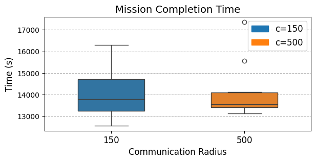
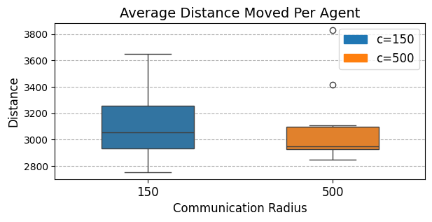
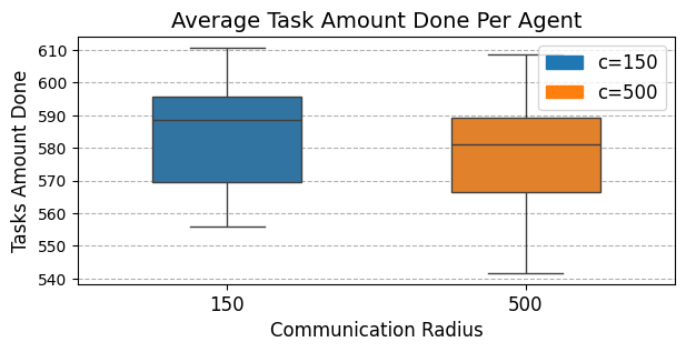